From Layered to General: How Virgo++ Broke the Linear Time Barrier in GKR

Introduction

Despite being introduced by Goldwasser et al.¹ as far back as 2008, the GKR protocol and its line of work remain among the most popular verifiable computation protocols today. In the Virgo++² paper by Zhang et al., the authors introduce a method to execute the GKR protocol for general circuits with linear proving time. In this post, we will discuss the techniques mentioned in the paper and provide some intuition on how they work. We encourage the readers to read the paper for further insights and to gain a complete view of the material mentioned in this blog post.

Improved Protocol

Before we dive into each of the changes, let’s take a look at the improved protocol to gain an overview of how it works. If you are already familiar with the original GKR protocol, you will notice that it looks almost the same. The main differences are:

1. The equations for each layer have been replaced with Equation 3.
2. The method for combining claims is implemented using a sum-check protocol as outlined in Equation 5.
3. Use the linear time sum-check algorithm.

Here’s a simplified view of Protocol 3 from the paper:

1. Define the function and compute the claim for the output at the layer $0$
   1. Define the multilinear extension of the circuit output as ${\tilde{V}}_0$.
   2. The verifier picks a random $g\in {\mathbb{F}}^{s_0}$ and send it to the prover.
   3. Both the verifier and the prover compute ${\tilde{V}}_0(g)$.
2. Round $i=0$
   1. The prover and the verifier run the sum-check protocol on Equation 3 for layer $i$.
   2. The verifier checks that ${\tilde{V}}_0(g)$ is the same as the prover’s claim in the last round of the sum-check protocol.
   3. The verifier now has the claims from the subsets of gates from all the layers connecting to layer $0$.
3. Round $i=1,\dots ,d$
   1. Combining the claims from the previous layer $i-1$
      1. The verifier picks $i+1$ random values and send them to the prover.
      2. The prover and verifier run the sum-check protocol on Equation 5 to combine the claims.
   2. if $i<d$, run the sum-check protocol on Equation 3 for layer $i$
      1. The prover and the verifier run the sum-check protocol on Equation 3 on the combined claims for layer $i$.
      2. The verifier checks that ${\tilde{V}}_i(g)$ is the same as the prover’s claim in the last round of the sum-check protocol.
      3. The verifier now has the claims from the subsets of gates from all the layers connecting to layer $i$.
4. Verify the input of the circuit
   1. The verifier is left with a claim of on the last layer $d$, ${\tilde{V}}_d(r^{(d)})$.
   2. The verifier can compute it locally or ask the oracle to verify the claim.

Let us now take a closer look at each of the changes.

Problem with GKR

One of the significant limitations of the original GKR protocol is that it can only work with layered arithmetic circuits. While in theory, any computations can be represented as a layered circuit, in practice, most computations are better represented as a general arithmetic circuit. Although a general circuit can be converted into a layered circuit by adding relay gates, this leads to a few problems:

1. The circuit size increases by a factor of $d$ (the depth of the circuit)
2. The prover time also increases by a factor of $d$, i.e. $O(d|C|)$
3. Common use cases, such as R1CS circuits, cannot be used directly as they need to be converted to layered circuits first

General Circuit vs Layered Circuit

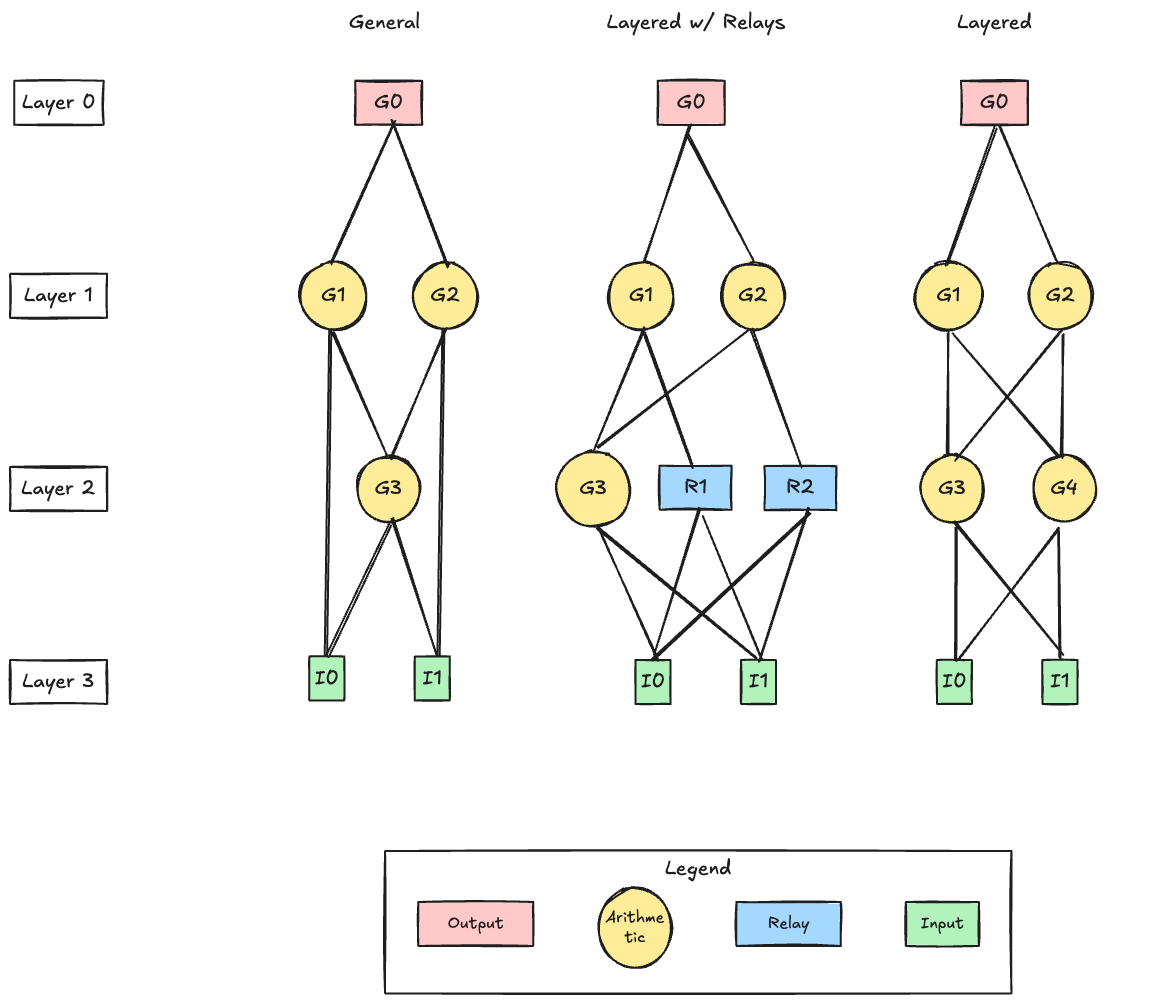
When discussing circuits in the GKR protocol, we refer to layered circuits as arithmetic circuits with gates of two inputs (fan-in 2) from the layer above. In contrast, general circuits have gates that can take inputs from any layers above.

General circuits can be converted into layered circuits simply by adding relay gates in the layers between any two connected gates in nonconsecutive layers. These relay gates simply forward the signals to the next level.

Before Virgo++, the fastest GKR-based protocol was Libra³, which has a prover time linear to the circuit size (i.e. $O(|C|)$) for layered circuits. Is there a way to apply the GKR protocol to general circuits also in $O(|C|)$?

Yes, of course, this is what we will be discussing next.

Generalizing the GKR protocol

To accept general circuits, the GKR protocol needs two main changes in the underlying sum-check protocol. Let’s examine each one.

Notation: Layers above and below

Throughout this blog post, we refer to the layers $i+1$ as being above the layer $i$, and layers $i-1$ as being below. Looking at the diagram, this may seem counterintuitive at first. However, you must realize that the diagram itself is also upside down because the layer $0$ is at the top and the layer $d$ is at the bottom.

We use this convention because it is consistent with the research papers that we have reviewed.

Problem #1: Considering Too Many Unused Connections

In GKR, the sum-check equation at each layer is only connected to outputs from the gates in the layer directly above because the circuits are layered. However, for general circuits, as each layer can take inputs from any layers above, the sum-check equation at each layer will have to consider the gates of every layer above.

For each layer $i$, there are summation terms of $\widetilde{add()}$ and $\widetilde{mult()}$ from layer $i+1$ to $d$ to represent the connections between layer $i$ to $d$. This is Equation 4 in the Virgo++ paper.

$$\begin{array}{rl}{\tilde{V}}_i(g)& =\sum _{x\in \{0,1{\}}^{s_{i+1}}}(\sum _{y\in \{0,1{\}}^{s_{i+1}}}\begin{array}{l}{\widetilde{\mathrm{add}}}_{i+1,i+1}(g,x,y)({\tilde{V}}_{i+1}(x)+{\tilde{V}}_{i+1}(y))\end{array}\}\text{between layer i and i+1}\\ & +\sum _{y\in \{0,1{\}}^{s_{i+2}}}\begin{array}{l}{\widetilde{\mathrm{add}}}_{i+1,i+2}(g,x,y)({\tilde{V}}_{i+1}(x)+{\tilde{V}}_{i+2}(y))\end{array}\}\text{between layer i and i+2}\\ & +\cdots +\sum _{y\in \{0,1{\}}^{s_d}}\begin{array}{l}{\widetilde{\mathrm{add}}}_{i+1,d}(g,x,y)({\tilde{V}}_{i+1}(x)+{\tilde{V}}_d(y))\end{array}\}\text{between layer i and d}\\ & +\sum _{y\in \{0,1{\}}^{s_{i+1}}}\begin{array}{l}{\widetilde{\mathrm{mult}}}_{i+1,i+1}(g,x,y)({\tilde{V}}_{i+1}(x){\tilde{V}}_{i+1}(y))\end{array}\}\text{between layer i and i+1}\\ & +\sum _{y\in \{0,1{\}}^{s_{i+2}}}\begin{array}{l}{\widetilde{\mathrm{mult}}}_{i+1,i+2}(g,x,y)({\tilde{V}}_{i+1}(x){\tilde{V}}_{i+2}(y))\end{array}\}\text{between layer i and i+2}\\ & +\cdots +\sum _{y\in \{0,1{\}}^{s_d}}\begin{array}{l}{\widetilde{\mathrm{mult}}}_{i+1,d}(g,x,y)({\tilde{V}}_{i+1}(x){\tilde{V}}_d(y))\end{array}\left)\right\}\text{between layer i and d}\end{array}\text{\hspace{1em}(1)}$$

In Equation 1, the equation considers the gates on a per-layer basis, rather than examining whether each gate is actually connected. When running the GKR protocol on the above equation, the prover needs to send to the verifier evaluations of ${\tilde{V}}_{i+1},...,{\tilde{V}}_d$ at random points after running the sum-check protocol at each layer. The resulting prover time is $O(d|C|)$. This is equivalent to converting a general circuit into a layered circuit by adding relay gates, as mentioned earlier. Surely there must be a better way.

Consider Only What Is Needed

In the circuits provided to the GKR protocol, each gate receives output from only two gates above. Thus, there should only be a maximum of 2 times the number of gates in the current layer to be considered for any layer above. We refer to these sets of gates connecting the layers above to the current layer as subsets. Thus, if we can adjust Equation 1 to only consider the subsets of gates from each of the layers above, we should have a much simpler equation. This is the idea behind our adjustments to Equation 1.

Here is the adjusted equation, which is Equation 6 in the paper:

$$\begin{array}{rl}{\tilde{V}}_i(g)=\sum _{x\in \{0,1{\}}^{s_{i+1}}}(& \begin{array}{l}\sum _{y\in \{0,1{\}}^{s_{i,i+1}}}{\widetilde{\mathrm{add}}}_{i+1,i+1}(g,x,y)({\tilde{V}}_{i,i+1}(x)+{\tilde{V}}_{i,i+1}(y))\end{array}\}\text{between subsets i and i+1}\\ +& \begin{array}{l}\sum _{y\in \{0,1{\}}^{s_{i,i+1}}}{\widetilde{\mathrm{mult}}}_{i+1,i+1}(g,x,y)({\tilde{V}}_{i,i+1}(x){\tilde{V}}_{i,i+1}(y))\end{array}\}\text{between subsets i and i+1}\\ +& \begin{array}{l}\sum _{y\in \{0,1{\}}^{s_{i,i+2}}}{\widetilde{\mathrm{add}}}_{i+1,i+2}(g,x,y)({\tilde{V}}_{i,i+1}(x)+{\tilde{V}}_{i,i+2}(y))\end{array}\}\text{between subsets i and i+2}\\ +& \begin{array}{l}\sum _{y\in \{0,1{\}}^{s_{i,i+2}}}{\widetilde{\mathrm{mult}}}_{i+1,i+2}(g,x,y)({\tilde{V}}_{i,i+1}(x){\tilde{V}}_{i,i+2}(y))\end{array}\}\text{between subsets i and i+2}\\ +& \dots \begin{array}{l}\sum _{y\in \{0,1{\}}^{s_{i,d}}}{\widetilde{\mathrm{add}}}_{i+1,d}(g,x,y)({\tilde{V}}_{i,i+1}(x)+{\tilde{V}}_{i,d}(y))\end{array}\}\text{between subsets i and d}\\ +& \dots \begin{array}{l}\sum _{y\in \{0,1{\}}^{s_{i,d}}}{\widetilde{\mathrm{mult}}}_{i+1,d}(g,x,y)({\tilde{V}}_{i,i+1}(x){\tilde{V}}_{i,d}(y))\end{array}\})\text{between subsets i and d}\end{array}\text{\hspace{1em}(2)}$$

Comparing Equation 2 to Equation 1, we can see that ${\tilde{V}}_i$, which refers to all the gates at layer $i$, has been replaced with ${\tilde{V}}_{i,j}$. ${\tilde{V}}_{i,j}$ refers to only the gates that connect between layer $i$ and $j$. The same definition changes apply for ${\widetilde{\mathrm{add}}}_{i,j}$, ${\widetilde{\mathrm{mult}}}_{i+1,i+2}$ and ${\sum }_{y\in \{0,1{\}}^{s_{i,j}}}$.

By considering only the used gates for each layer, the size of ${\tilde{V}}_{i,i+1},...,{\tilde{V}}_{i,d}$ is now $O(S_i)$ instead of $O(S_i+S_{i+1}+\cdots +S_d)$ like before. We will see later on how this helps us with improving the prover time to $O(S_i)$.

Eliminating the Inner Sums

In Equation 2, for each layer $i$ it involves a grand sum ${\sum }_{x\in \{0,1{\}}^{s_{i+1}}}$ over many inner sums that include the $\widetilde{add}$ and $\widetilde{mult}$ predicates for each subset of gates between layer $i$ and the layers above. To simplify this equation for efficient execution during the sum-check protocol, we need to reduce it to a single sum.

Currently, each of the inner sums has different bit lengths depending on the number of gates in the subset. To remove the inner sums, we will select the longest binary string in the circuit, denoted as $y\in \{0,1{\}}^{s_{i,i+1}}$, and force all inner sums to run over it.

Ensuring Shorter Polynomials Are Summed Only Once

When all the inner sums are run over the same binary string, the binary strings that have shorter lengths may be summed multiple times because of the extra padding. To ensure they are only summed over once, we can multiply each of the predicates by the binary string $y_{s_{i,j+1}}\cdot y_{s_{i,j+2}}\cdot \dots \cdot y_{s_{i,i+1}}$.

Final Sum-Check Equation For Layer $i$

Taking into account of the above 2 points, we are ready to adjust Equation 2 by removing the inner sums and adding the binary string $y_{s_{i,j+1}}\cdot y_{s_{i,j+2}}\cdot \dots \cdot y_{s_{i,i+1}}$ as below (which is Equation 7 in the paper):

$$\begin{array}{rl}{\tilde{V}}_i(g)=\sum _{x,y\in \{0,1{\}}^{s_{i,i+1}}}(& {\widetilde{\mathrm{add}}}_{i+1,i+1}(g,x,y)({\tilde{V}}_{i,i+1}(x)+{\tilde{V}}_{i,i+1}(y_1,\dots ,y_{s_{i,i+1}}))\\ & +y_{s_{i,i+2}+1}\cdot \dots \cdot y_{s_{i,i+1}}{\widetilde{\mathrm{add}}}_{i+1,i+2}(g,x,y_1,\dots ,y_{s_{i,i+2}})({\tilde{V}}_{i,i+1}(x)+{\tilde{V}}_{i,i+2}(y_1,\dots ,y_{s_{i,i+2}}))\\ & +\cdots +y_{s_{i,d}+1}\cdot \dots \cdot y_{s_{i,i+1}}{\widetilde{\mathrm{add}}}_{i+1,d}(g,x,y_1,\dots ,y_{s_{i,d}})({\tilde{V}}_{i,i+1}(x)+{\tilde{V}}_{i,d}(y_1,\dots ,y_{s_{i,d}}))\\ & +{\widetilde{\mathrm{multi}}}_{i+1,i+1}(g,x,y){\tilde{V}}_{i,i+1}(x){\tilde{V}}_{i,i+1}(y_1,\dots ,y_{s_{i,i+1}})\\ & +y_{s_{i,i+2}+1}\cdot \dots \cdot y_{s_{i,i+1}}{\widetilde{\mathrm{multi}}}_{i+1,i+2}(g,x,y_1,\dots ,y_{s_{i,i+2}}){\tilde{V}}_{i,i+1}(x){\tilde{V}}_{i,i+2}(y_1,\dots ,y_{s_{i,i+2}})\\ & +\cdots +y_{s_{i,d}+1}\cdot \dots \cdot y_{s_{i,i+1}}{\widetilde{\mathrm{multi}}}_{i+1,d}(g,x,y_1,\dots ,y_{s_{i,d}}){\tilde{V}}_{i,i+1}(x){\tilde{V}}_{i,d}(y_1,\dots ,y_{s_{i,d}}))\end{array}\text{\hspace{1em}(3)}$$

Example

Here is an example to illustrate the above two ideas:

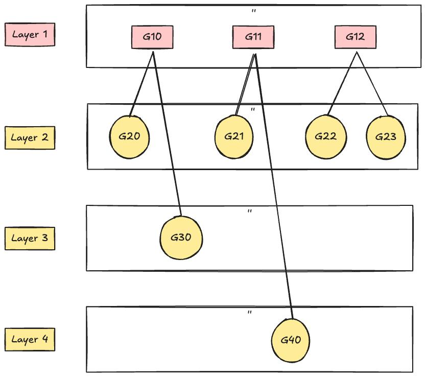
Layer $j$	Gates Feeding $g_{10}$	Padded Size	Bit-length $s_{1,j}$
$2$	4 gate ($g_{20},g_{21},g_{22},g_{23}$)	4	$s_{1,2}=2$
$3$	1 gate ($g_{30}$)	2	$s_{1,3}=1$
4	1 gate ($g_{40}$)	2	$s_{1,4}=1$

The above circuit will give us 3 inner sums:

$$\underset{\text{subset 2 term}}{\underbrace{\sum _{y\in \{0,1{\}}^{s_{1,2}}}{F}_{1,2}(y)}}+\underset{\text{subset 3 term}}{\underbrace{\sum _{y\in \{0,1{\}}^{s_{1,3}}}{F}_{1,3}(y)}}+\underset{\text{subset 4 term}}{\underbrace{\sum _{y\in \{0,1{\}}^{s_{1,4}}}{F}_{1,4}(y)}}\text{\hspace{1em}(4)}$$

where $F_j(y)$ represent the outputs of the $\widetilde{add}$ and $\widetilde{mult}$ gates in the subset for the layer $j$.

Since the longest binary string is from layer 2 with 4 gates, we will set $y$ as $s_{1,2}=2\Rightarrow \{0,1{\}}^2$.

The above 3 subsets will give us 3 inner sums run over the same binary string of $\{0,1{\}}^2$:

For each of the sums, we will multiply by the appropriate binary string $y_{s_{i,j+1}}\cdot y_{s_{i,j+2}}\cdot \dots \cdot y_{s_{i,i+1}}$ to ensure it doesn’t get summed over multiple times.

Layer	Bit-length	Binary String to Add	Summation Occurs	Summation Avoided
2	2	none	-	-
3	1	$y_{s_{1,3}+1}$	$y_{s_{1,3}+1}=1$, which gives: $1\cdot F_{1,3}(y_1,\dots ,y_{s_{1,3}})$	$y_{s_{1,3}+1}=0$, which gives: $0\cdot F_{1,3}(y_1,\dots ,y_{s_{1,3}})$
4	1	$y_{s_{1,4}+1}$	$y_{s_{1,4}+1}=1$, which gives: $1\cdot F_{1,4}(y_1,\dots ,y_{s_{1,4}})$	$y_{s_{1,4}+1}=0$, which gives: $0\cdot F_{1,4}(y_1,\dots ,y_{s_{1,4}})$

$$\sum _{(x,y)\in \{0,1{\}}^{s_{1,2}}}(F_{1,2}(y_1,\dots ,y_{s_{1,2}})+y_{s_{1,3}+1}{F}_{1,3}(y_1,\dots ,y_{s_{1,3}})+y_{s_{1,4}+1}{F}_{1,4}(y_1,\dots ,y_{s_{1,4}}))$$

This equation of a grand sum over the Boolean hypercube $\{0,1{\}}^2$ is equivalent to the 3 separate sums in Equation 4.

Problem #2: Combining claims efficiently

Remember that in the original GKR protocol, the verifier uses the sum-check protocol to check that the following equation is computed correctly:

$$\begin{array}{rlrl}\widetilde{V_i}(g)& =\sum _{x,y\in {0,1}^{s_{i+1}}}& & f_i(g,x,y)\\ & =\sum _{x,y\in {0,1}^{s_{i+1}}}& & {\widetilde{add}}_{i+1}(g,x,y)({\tilde{V}}_{i+1}(x)+{\tilde{V}}_{i+1}(y))\\ & & & +{\widetilde{mult}}_{i+1}(g,x,y)({\tilde{V}}_{i+1}(x)+{\tilde{V}}_{i+1}(y))\end{array}$$

where $g\in {\mathbb{F}}^{s_i}$ is a random vector, $x$ and $y$ are random values in ${\mathbb{F}}^{s_{i+1}}$.

When the sum-check protocol for the layer $i=0$ is finished, the verifier needs to compute $f_0(g,x,y)$. To do this, the verifier computes ${\widetilde{add}}_1(g,x,y)$ and ${\widetilde{mult}}_1(g,x,y)$, and ask the prover to send $\widetilde{V_1}(x)$ and $\widetilde{V_1}(y)$. Thus, a claim about the output value, $\widetilde{V_0}$ in layer $0$, is reduced to two claims $\widetilde{V_1}(x)$ and $\widetilde{V_1}(y)$ in layer $1$. The sum-check protocol would repeat on each of the two claims until the claims are reduced to the input layers. You can see that this increases the number of sum-check protocols exponentially with the number of layers.

But recall that we can use a random linear combination to combine the two claims:

$${\alpha }_1{\tilde{V}}_1(x)+{\alpha }_2{\tilde{V}}_1(y)$$

where ${\alpha }_1,{\alpha }_2\in \mathbb{F}$ are random values.

The prover and verifier can then execute the sum-check protocol on the random linear combination of claims once and receive claims about the next layer.

Cannot Combine Claims From the New Equation

When we generalize GKR to general circuits, we obtain a new equation (Equation 3) to run the sum-check protocol on. Recall that this equation sums subsets of gates from all the layers above that are connected to the current layer. This means that when the sum-check protocol is finished, we will be left with multiple evaluations of different multilinear extensions defined by subsets from different layers. This invalidates the random linear combination method we previously used, and we must find an alternative method to efficiently combine these evaluation claims.

Sum-check Protocol To The Rescue

As it turns out, the best way to combine these evaluations is through a (yet another) sum-check protocol on an equation that uses a random linear combination. The following is Equation 10 from the paper. Let’s break it down and see how it works.

$$\begin{array}{rl}& \sum _{k=0}^{i-1}{\alpha }_{k,i}\underset{\text{subsets of layers up to i−1}}{\underbrace{{\tilde{V}}_{k,i}\left(r^{(k,i)}\right)}}+{\alpha }_{i-1,i}^{\prime }{\tilde{V}}_{i-1,i}\left(r^{(i-1,i{)}^{\prime }}\right)\\ & =\sum _{k=0}^{i-1}{\alpha }_{k,i}\left(\sum _{x\in \{0,1{\}}^{s_i}}\underset{\text{=1 iff 2 inputs are from same gate}}{\underbrace{{\tilde{C}}_{k,i}(r^{(k,i)},x)}}{\tilde{V}}_i(x)\right)+{\alpha }_{i-1,i}^{\prime }\sum _{x\in \{0,1{\}}^{s_i}}\underset{\text{=1 iff 2 inputs are from same gate}}{\underbrace{{\tilde{C}}_{i-1,i}(r^{(i-1,i{)}^{\prime }},x)}}{\tilde{V}}_i(x)\\ & =\sum _{x\in \{0,1{\}}^{s_i}}{\tilde{V}}_i(x)\left(\sum _{k=0}^{i-1}{\alpha }_{k,i}{\tilde{C}}_{k,i}(r^{(k,i)},x)+{\alpha }_{i-1,i}^{\prime }{\tilde{C}}_{i-1,i}(r^{(i-1,i{)}^{\prime }},x)\right)\\ & =\sum _{x\in \{0,1{\}}^{s_i}}{\tilde{V}}_i(x)\underset{\text{computed by verifier}}{\underbrace{g_i(x)}}\end{array}\text{\hspace{1em}(5)}$$

where ${\alpha }_{0,i},\dots ,{\alpha }_{i-1,i},{\alpha }_{i_1,1}^{\prime }$ are random values chosen by the verifier for each layer $i$.

In the first line of Equation 5, we can see that there is a summation of a random linear combination of two evaluations, one from the subsets of layers below $i-1$, and two from layer $i-1$.

To combine the evaluations, we introduce a new function $C_{k,i}(z,x)$ that equals 1 only if the gate $z$ in the subset $V_{k,i}$ is the same as gate $x$ in layer $i$. Since we are dealing with multilinear extensions, we want ${\tilde{C}}_{k,i}(r^{k,i)},x)$, which only equals 1 if $r^{k,i}$ in the subset $V_{k,i}$ is the same gate as $x$ from layer $i$. This function helps to rewrite the equation only in terms of $V_i$ as seen in line 2 of Equation 5.

By further rearranging lines 2 to 3 and 4, we obtain an expression, $g_i(x)$, that only depends on the circuit structure and can be computed by the verifier given $r^{\{i\}}$.

Now that we have Equation 5, we can use the same linear-time sum-check algorithm used earlier for each layer of our modified GKR protocol (Equation 3).

Linear-time Sum-check Algorithm (To Be Complete)

Let’s review what we have so far:

1. To reduce the complexity of the layer $i$ equation, we introduce subsets and rewrite Equation 1 into Equation 2 and finally into Equation 3 to be computed using the sum-check protocol.
2. To combine the claims efficiently, we introduce Equation 5, which is also intended for the sum-check protocol.

Given the importance of the sum-check protocol, it is only fitting that we have an efficient algorithm to run it.

The sum-check protocol used in the original GKR paper has a prover time of $O(|C{|}^2)$, which is far from ideal. Luckily, we have a better algorithm. Originally introduced in the Libra paper³, the sum-check algorithm there has a prover time of $O(|C|)$. Thus, applying this efficient sum-check algorithm on our two equations will also give us a linear prover time. While the explanation of this algorithm is out of scope for this post, readers can refer to the paper for a full understanding of how it works.

Conclusion

What makes Virgo++ particularly elegant is how it solves the general circuit problem without fundamentally changing the GKR protocol’s structure. By recognizing that most gates in upper layers are irrelevant to any given gate below, and by using the sum-check protocol not just for the main computation but also for combining claims, the authors achieve something that seemed inherently quadratic in just $O(|C|)$ time. The protocol maintains the same security guarantees as the original GKR while being dramatically more efficient. For practitioners, this means you can now apply GKR directly to your existing circuit representations without worrying about the dd d-factor blowup from adding relay gates—a game-changer for verifiable computation in practice.

Reference

Footnotes

1. Delegating Computation: Interactive Proofs for Muggles by Goldwasser et al. (2008) ↩

2. Doubly Efficient Interactive Proofs for General Arithmetic Circuits with Linear Prover Time (a.k.a. Virgo++) by Zhang et al., (2021) ↩

3. Libra: Succinct Zero-Knowledge Proofs with Optimal Prover Computation by Xie et al. (2019) ↩ ↩²